Monotone Piecewise Cubic Interpolation in SQL Server
Aug
22
Written by:
Charles Flock
8/22/2013 4:39 PM

We have added a new function, MONOSPLINE, to the XLeratorDB/math 2008 library based on "Monotone Piecewise Cubic Interpolation," by Fritsch, F. N. and R. E. Carlson, SIAM J. Numerical Analysis, Vol. 17, 1980, pp.238-246. In this article we look at how the MONOSPLINE function works on monotonic data and compare it to linear, natural cubic spline, and polynomial interpolation in SQL Server.
I think of interpolation as a method of approximating reality. On other words, given a series of points, x and y, it is possible to fill in the gaps in a meaningful way by using interpolation. In other words, given some point, a, lying between xi and xi+1, calculate a value, ß, lying between yi and yi+1. It is actually quite surprising to me that given how useful interpolation functions are and how often even rudimentary calculations require an interpolated value that interpolation functions are not part of packages like EXCEL and SQL Server.
The simplest (and fastest) interpolation method is linear interpolation. Linear interpolation treats every interval, xi and xi+1, as a line having a slope (d) of (yi+1-yi)/(xi+1-x1). Thus, for any value a, lying between xi and xi+1, the value ß is calculated as ß = yi + (a -xi)* d.
Linear interpolation is implemented in the XLeratorDB INTERP function. We will use the data from the Fritsch and Carlson paper for demonstration purposes. In this example, we will return the interpolated value for y when x is equal to 8.5.
SELECT wct.INTERP(x,y,8.5) as [Linear]
FROM (VALUES
(7.99,0),
(8.09,2.76429E-05),
(8.19,4.37498E-02),
(8.7,0.169183),
(9.2,0.469428),
(10,0.943740),
(12,0.998636),
(15,0.999919),
(20,0.999994)
)n(x,y)
This produces the following result.
Linear
----------------------
0.119993509803922
For purpose of this article, however, we are more interested in the overall shape of the values returned by the interpolating function. Thus, our next piece of SQL will calculate a y-value for each x between 7.99 and 20.0 in steps of 0.01. We will then take the resultant table and dump the results into EXCEL and graph the results.
SELECT k.seriesvalue
,wct.INTERP(x,y,k.seriesvalue) as [Linear]
FROM (VALUES
(7.99,0),
(8.09,2.76429E-05),
(8.19,4.37498E-02),
(8.7,0.169183),
(9.2,0.469428),
(10,0.943740),
(12,0.998636),
(15,0.999919),
(20,0.999994)
)n(x,y)
CROSS APPLY wct.SeriesFloat(7.99,20,0.01,NULL,NULL)k
GROUP BY k.seriesvalue
Here is the graph of the resultant table.
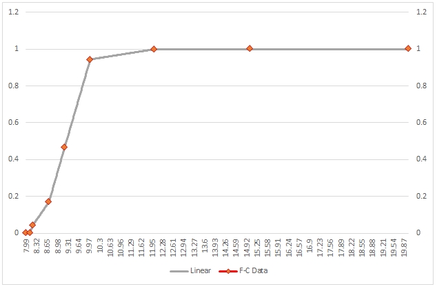
As you can see, the interpolated values between any two x-values are calculated as a straight line and the overall shape of interpolated values is simply a series of connected line segments. This shape is simply a manifestation of the fact that linear interpolation does not consider the overall shape of the data.
Polynomial interpolation is only concerned with the shape of the data and makes no effort to make sure that any interpolated point intersects existing data points. Polynomial interpolation calculates a polynomial of the specified degree which “best fits” the data points. Polynomial interpolation is implemented in the XLeratorDB POLYVAL function.
SELECT k.seriesvalue
,wct.POLYVAL(x,y,3,k.seriesvalue) as [Polynomial]
FROM (VALUES
(7.99,0),
(8.09,2.76429E-05),
(8.19,4.37498E-02),
(8.7,0.169183),
(9.2,0.469428),
(10,0.943740),
(12,0.998636),
(15,0.999919),
(20,0.999994)
)n(x,y)
CROSS APPLY wct.SeriesFloat(7.99,20,0.01,NULL,NULL)k
GROUP BY k.seriesvalue
Here is a graph of the resultant table.
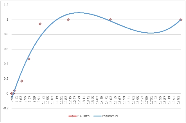
While the polynomial interpolation certainly produces a smoother curve of the interpolated values, it oscillates both above and below the y-values. In other words, it interpolates a y-value less than the minimum y-value (0) as well as interpolating values greater than the maximum y-value (0.999994). It not only does this globally, but it also locally, meaning that any interval xi to xi+1 the interpolating function is not bound by yi and yi+1, which is apparent from the graph.
Cubic splines are a way of interpolating values using the shape of the data as part of the interpolating function. The math of this is beyond the scope of this article. Cubic spline interpolation is implemented in the XLeratorDB SPLINE function.
SELECT k.seriesvalue
,wct.SPLINE(x,y,k.seriesvalue) as [SPLINE]
FROM (VALUES
(7.99,0),
(8.09,2.76429E-05),
(8.19,4.37498E-02),
(8.7,0.169183),
(9.2,0.469428),
(10,0.943740),
(12,0.998636),
(15,0.999919),
(20,0.999994)
)n(x,y)
CROSS APPLY wct.SeriesFloat(7.99,20,0.01,NULL,NULL)k
GROUP BY k.seriesvalue
Here is a graph of the resultant table.
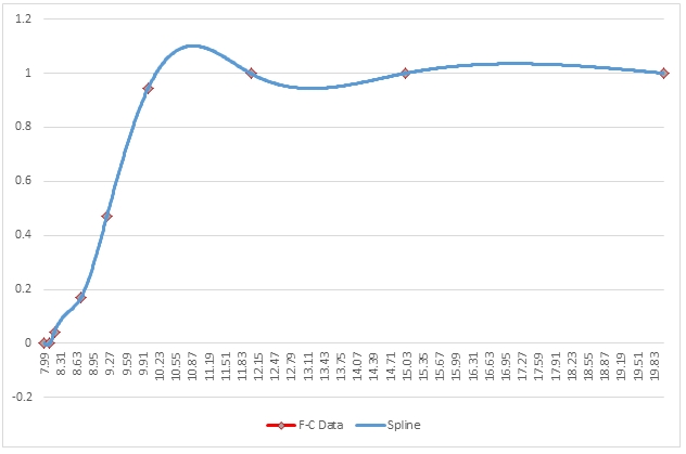
Here we can see that the shape of the interpolated points is smoother than what was seen in the linear interpolation and that the interpolated values go through the existing data points which was not the case with polynomial interpolation. However, we can still see that there are oscillation problems similar to the ones that we noticed with polynomial interpolation.
Now, let’s look at monotonic cubic spline interpolation. This type of interpolation constructs a monotone piecewise interpolant to monotone data. In other words, it considers the shape of the data but then modifies the interpolants to eliminate the oscillations (or bumps and wiggles as they are referred to by Fritsch and Carlson). The method delineated by Fritsch and Carlson is implemented in the XLeratorDB MONOSPLINE function.
SELECT k.seriesvalue
,wct.MONOSPLINE(x,y,k.seriesvalue) as [MONOTONIC SPLINE]
FROM (VALUES
(7.99,0),
(8.09,2.76429E-05),
(8.19,4.37498E-02),
(8.7,0.169183),
(9.2,0.469428),
(10,0.943740),
(12,0.998636),
(15,0.999919),
(20,0.999994)
)n(x,y)
CROSS APPLY wct.SeriesFloat(7.99,20,0.01,NULL,NULL)k
GROUP BY k.seriesvalue
Here is a graph of the resultant table.
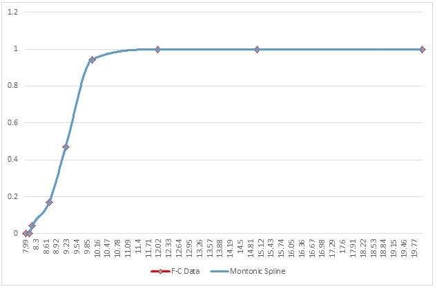
The monotonic spline interpolation demonstrates the smoothness of the cubic spline interpolation but has eliminated the bumps and wiggles. Let’s compare the monotonic spline and the cubic spline.
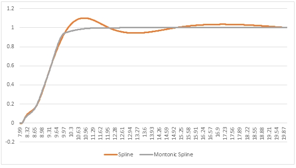
As you can see, the monotonic spline has all the smoothness of the cubic spline but avoids the overshoot and the undershoot when x > 9.2
In this particular example, though, the linear interpolation and the monotonic cubic spline interpolation returned graphs that seemed pretty similar in shape. Let’s compare them.
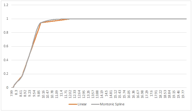
As you can see, there is not a great deal difference between the 2 graphs, though we can zoom in a little bit on the area where x is between 9.2 and 10.0. That area looks like this.
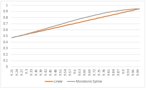
Both interpolations go through the same point at 9.2 and 10.0 but the monotonic cubic spline interpolation is curved based upon the values before 9.20 and after 10.0 whereas the linear interpolation has a constant slope in this interval.
No one interpolation function is right for every occasion and the monotonic spline function is best used for monotonic data, though it is not limited to that use. Clearly, linear interpolation is not a bad approximation for monotonic data, but it is going to perform best when used on linear data.
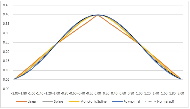
Here’s an example where have calculated the values for the probability density function of the standard normal distribution and then performed the interpolation using all the methods and graphed the results.
SELECT k.SeriesValue as x
,wct.INTERP(p.seriesvalue,wct.NORMAL(p.seriesvalue),k.seriesvalue) as [Linear]
,wct.SPLINE(p.seriesvalue,wct.NORMAL(p.seriesvalue),k.seriesvalue) as [Spline]
,wct.MONOSPLINE(p.seriesvalue,wct.NORMAL(p.seriesvalue),k.seriesvalue) as [Monotonic Spline]
,wct.POLYVAL(p.seriesvalue,wct.NORMAL(p.seriesvalue),8,k.seriesvalue) as [Polynomial]
,wct.NORMAL(k.SeriesValue) as [Normal pdf]
FROM wct.SeriesInt(-4,4,1,NULL,NULL)p
CROSS APPLY wct.SeriesFloat(-4,4,0.1,NULL,NULL)k
GROUP BY k.SeriesValue
Here is a graph of the resultant table.
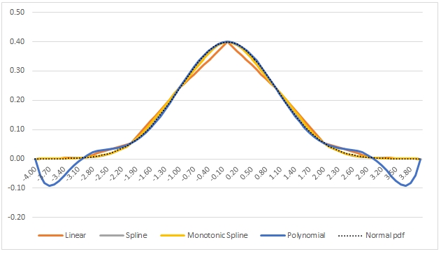
As you can see, all of the interpolations provide a pretty good fit, but the monotonic spline and the cubic spline seem to have the best overall fit. However, in the region ±2 (standard deviations), the polynomial interpolation technique seems to provide an almost perfect fit.
The MONOSPLINE function is another tool that makes SQL Server a powerful analytic platform supporting sophisticated data analysis directly on the database without having to send the data over the network. All you need to know to do these kinds of calculations on your data is some basic SQL. We developed this function based on a user request, so if there is some function you would like to see added to SQL Server, please let us know.