Calculating FIFO balances in SQL Server
Feb
26
Written by:
Charles Flock
2/26/2013 6:27 PM

With the release of XLeratorDB/windowing 1.01 we introduce three new functions for calculating inventory values: FIFO; LIFO; and WAC. These functions calculate the quantity-on-hand, cost-of-goods sold, gross margin, and inventory value using the First In, First Out (FIFO), Last In, First Out (LIFO), or Weighted Average Cost (WAC) method. In this article we talk about how those calculations work and how you can incorporate these calculations into T-SQL statements without having to do a self-join.
The calculation of inventory values is a straightforward arithmetic calculation, but can be quite difficult in T-SQL as it requires information from previous rows to calculate a value for the current row. Additionally, for many financial calculations inventory may be positive or negative as it is possible to be short a stock, bond, currency, commodity, or some other financial instrument.
While there are many different values that might be produced in an inventory report, we are going to focus on four: quantity on hand, inventory value, cost-of-goods sold, and gross margin. For the purposes of this article, when examining these calculations we will be making the following assumption: a quantity added to inventory is either unsigned or has a plus sign; a quantity subtracted from inventory has a minus sign; the monetary value of the quantity has the same sign as the quantity.
We also need to define a couple of other calculations. The cost-of goods sold is equal to Ending Inventory – (Beginning Inventory + Purchases). The gross margin is equal to the Invoice Amount – Cost of Goods Sold.
The FIFO (First In, First Out) method provides an inventory valuation based on the assumption that the inventory on-hand is comprised of the goods that were received most recently. This is simply an assumption about the inventory and has nothing to with the actual movement of the inventory. In a period of rising prices for inventory, the FIFO method has the effect of decreasing the cost-of-goods sold, thereby increasing income. In periods of declining prices for inventory, the FIFO method increases the cost-of-goods sold, decreasing income. You can see this in the table below.
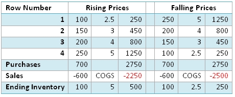
As you can see, the total purchases are the same. However, the value of the ending inventory for the Rising Prices is 500 which is 100 units of the fourth row at a cost of 5, while the ending inventory for the Falling Prices is 250, which is 100 units of the fourth row at a cost of 2.50. The difference manifests itself of the cost-of goods sold (COGS), which is a deduction from revenue. In the Rising Prices case, the deduction from revenue is less than it is in the Falling Prices case.
The LIFO (Last In, First Out) method provides a valuation for your inventory based on the assumption that the cost of goods sold is comprised of the goods that were received most recently. In a period of rising prices for inventory, the LIFO method has the effect of increasing the cost-of-goods sold, thereby decreasing income. In periods of declining prices for inventory, the LIFO method decreases the cost-of-goods sold, increasing income. You can see this in the table below.
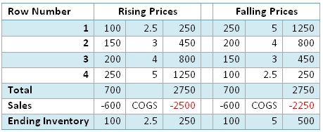
Compared to the FIFO inventory example, we can see that LIFO produced exactly the opposite result.
As we will see in some of the T-SQL examples, LIFO can be pretty tricky because once an item has been removed from inventory it cannot be added back in. In other words, you cannot just sum the additions to inventory from the beginning of the dataset until you get to the quantity on-hand. You have to apply the additions and withdrawals from inventory in the proper order.
The weighted average cost calculation is much simpler. It is simply the weighted average cost of the additions to inventory up until the time that an item is withdrawn from inventory. When the quantity on hand goes to zero, the weighted average cost is zero. Using the same data as above, here are the results using weighted average cost.
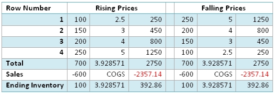
As you can see, the weighted average cost of the inventory is the same for both rising prices and falling prices.
To compare the results of the calculations among the three methods, let’s create a table and put some data in it. For illustration purposes, we will start with some purchase and sale transactions in the shares of the XYZ Corporation.
CREATE TABLE #c(
trn int,
tDate date,
qty money,
price_share money,
price_extended money
)
INSERT INTO #c VALUES (91908,'2013-01-02',600,95.35,57210)
INSERT INTO #c VALUES (94967,'2013-01-04',-300,103.34,-31002)
INSERT INTO #c VALUES (56450,'2013-01-04',300,99.69,29907)
INSERT INTO #c VALUES (57542,'2013-01-09',100,95.94,9594)
INSERT INTO #c VALUES (64078,'2013-01-10',-400,96.88,-38752)
INSERT INTO #c VALUES (14025,'2013-01-19',-300,104.51,-31353)
INSERT INTO #c VALUES (97117,'2013-02-04',900,99.3,89370)
INSERT INTO #c VALUES (67549,'2013-02-05',-500,104.14,-52070)
INSERT INTO #c VALUES (79673,'2013-02-21',400,99.36,39744)
INSERT INTO #c VALUES (58627,'2013-02-25',-600,97.29,-58374)
Let’s look at the inventory valuation calculations, starting with the FIFO function. Like all XLeratorDB / windowing functions, we will use the SQL Server ROW_NUMBER()function to return data in the required order.
SELECT ROW_NUMBER() OVER (ORDER BY tDate, qty ASC) as rn
,tDate
,qty
,price_share as price
,price_extended as basis
,wct.FIFO(qty, price_extended,'QTY',2,ROW_NUMBER() OVER (ORDER BY tDate, qty ASC), 0) as Shares
,wct.FIFO(qty, price_extended,'EV',2,ROW_NUMBER() OVER (ORDER BY tDate, qty ASC), 1) as Value
FROM #c
This produces the following result.
rn tDate qty price basis Shares Value
---- ---------- ---- ------ --------- ------ ----------
1 2013-01-02 600 95.35 57210.00 600 57210.00
2 2013-01-04 -300 103.34 -31002.00 300 28605.00
3 2013-01-04 300 99.69 29907.00 600 58512.00
4 2013-01-09 100 95.94 9594.00 700 68106.00
5 2013-01-10 -400 96.88 -38752.00 300 29532.00
6 2013-01-19 -300 104.51 -31353.00 0 .00
7 2013-02-04 900 99.30 89370.00 900 89370.00
8 2013-02-05 -500 104.14 -52070.00 400 39720.00
9 2013-02-21 400 99.36 39744.00 800 79464.00
10 2013-02-25 -600 97.29 -58374.00 200 19872.00
Let’s look at how the inventory amounts are calculated. In the first row, the inventory value is the extended price (price * quantity) of the first transaction. This will always be the case for the first row in a partition, regardless of the inventory method. Thus the transaction amount and the inventory amount are the same.
In the second row, we are selling 300 shares, or half of the inventory. That amount is subtracted from the inventory. The third and fourth rows are additions to inventory; we can simply add those amounts to the half of our original inventory amount from the first row,
68,106 = 28,605 + 29,907 + 9,594
In the fifth row, we are selling 400 shares, leaving 300 in inventory. Since this is the FIFO method, the value of the inventory will be calculated from the most recent row back.
29,532 = 100 * 95.94 + 200 * 99.69
In the sixth row, we sell all the remaining shares that we own, reducing the inventory balance to zero. Whenever the quantity-on-hand is zero, the inventory balance is zero.
This process is repeated for all the subsequent rows.
Let’s contrast this calculation with the LIFO calculation. We can simply add one more line to our SQL to bring in the LIFO values.
SELECT ROW_NUMBER() OVER (ORDER BY tDate, qty ASC) as rn
,tDate
,qty
,price_share as price
,price_extended as basis
,wct.FIFO(qty, price_extended,'QTY',2,ROW_NUMBER() OVER (ORDER BY tDate, qty ASC), 0) as Shares
,wct.FIFO(qty, price_extended,'EV',2,ROW_NUMBER() OVER (ORDER BY tDate, qty ASC), 1) as FIFO
,wct.LIFO(qty, price_extended,'EV',2,ROW_NUMBER() OVER (ORDER BY tDate, qty ASC), 0) as LIFO
FROM #c
This produces the following result.
rn tDate qty price basis Shares FIFO LIFO
---- ---------- ---- ------ --------- ------ ---------- ----------
1 2013-01-02 600 95.35 57210.00 600 57210.00 57210.00
2 2013-01-04 -300 103.34 -31002.00 300 28605.00 28605.00
3 2013-01-04 300 99.69 29907.00 600 58512.00 58512.00
4 2013-01-09 100 95.94 9594.00 700 68106.00 68106.00
5 2013-01-10 -400 96.88 -38752.00 300 29532.00 28605.00
6 2013-01-19 -300 104.51 -31353.00 0 .00 .00
7 2013-02-04 900 99.30 89370.00 900 89370.00 89370.00
8 2013-02-05 -500 104.14 -52070.00 400 39720.00 39720.00
9 2013-02-21 400 99.36 39744.00 800 79464.00 79464.00
10 2013-02-25 -600 97.29 -58374.00 200 19872.00 19860.00
As you can see, through the first four rows, the calculations are the same. In row 5, however, the value of the inventory is obtained from the oldest inventory row forward. As we calculated above, the LIFO value in row 4 is 68,106 and the number of shares is 700. The LIFO calculation in row 5 removes the most recent addition to inventory.
28,605 = 68,106 – 100 * 95.94 – 300 * 99.69
The important thing to remember is that these rows have been removed, never to return, and additions to inventory start from the values that remain in inventory.
Thus when looking at the seventh row, where we have added 900 shares at a price of 99.30, the value of inventory is 89,370 consisting entirely of the items just added to the inventory. It does not consist of 600 shares from the first row and 300 shares from the third row as those shares had already been removed from inventory.
Let’s add the weighted-average cost calculation to our SQL.
SELECT ROW_NUMBER() OVER (ORDER BY tDate, qty ASC) as rn
,tDate
,qty
,price_share as price
,price_extended as basis
,wct.FIFO(qty, price_extended,'QTY',2,ROW_NUMBER() OVER (ORDER BY tDate, qty ASC), 0) as Shares
,wct.FIFO(qty, price_extended,'EV',2,ROW_NUMBER() OVER (ORDER BY tDate, qty ASC), 1) as FIFO
,wct.LIFO(qty, price_extended,'EV',2,ROW_NUMBER() OVER (ORDER BY tDate, qty ASC), 0) as LIFO
,wct.WAC(qty, price_extended,'EV',2,ROW_NUMBER() OVER (ORDER BY tDate, qty ASC), 0) as WAC
FROM #c
This produces the following result.
rn tDate qty price basis Shares FIFO LIFO WAC
---- ---------- ---- ------ --------- ------ ---------- ---------- ----------
1 2013-01-02 600 95.35 57210.00 600 57210.00 57210.00 57210.00
2 2013-01-04 -300 103.34 -31002.00 300 28605.00 28605.00 28605.00
3 2013-01-04 300 99.69 29907.00 600 58512.00 58512.00 58512.00
4 2013-01-09 100 95.94 9594.00 700 68106.00 68106.00 68106.00
5 2013-01-10 -400 96.88 -38752.00 300 29532.00 28605.00 29188.29
6 2013-01-19 -300 104.51 -31353.00 0 .00 .00 .00
7 2013-02-04 900 99.30 89370.00 900 89370.00 89370.00 89370.00
8 2013-02-05 -500 104.14 -52070.00 400 39720.00 39720.00 39720.00
9 2013-02-21 400 99.36 39744.00 800 79464.00 79464.00 79464.00
10 2013-02-25 -600 97.29 -58374.00 200 19872.00 19860.00 19866.00
As with LIFO, there is no difference from the FIFO calculation through the first four rows. However, in row five, 400 shares are removed from inventory at the weighted average cost.
29,188.29 = 300/700 * 68,106
As with the LIFO calculation, once those shares are removed from the inventory calculation, they never return.
In the seventh row, then, the inventory is made up entirely of the 900 shares added by that transaction, as the inventory was depleted by the previous transaction, removing all the previous values from the inventory calculation. In fact, the values for the seventh row are the same for all three valuation methods because the inventory went to zero on the previous row.
Now that we know how the inventory balances are calculated, let’s look at how cost-of-goods sold and gross margin are calculated. The calculations are the same regardless of inventory method, so we will use FIFO in our example. Using the data in the #c table, the following SQL will return the quantity-on-hand, inventory value, cost-of-goods sold, and gross margin.
SELECT ROW_NUMBER() OVER (ORDER BY tDate, qty ASC) as rn
,tDate
,qty
,price_share as price
,price_extended as basis
,wct.FIFO(qty, price_extended,'QTY',2,ROW_NUMBER() OVER (ORDER BY tDate, qty ASC), 0) as Shares
,wct.FIFO(qty, price_extended,'EV',2,ROW_NUMBER() OVER (ORDER BY tDate, qty ASC), 1) as Value
,wct.FIFO(qty, price_extended,'COGS',2,ROW_NUMBER() OVER (ORDER BY tDate, qty ASC), 2) as COGS
,wct.FIFO(qty, price_extended,'GM',2,ROW_NUMBER() OVER (ORDER BY tDate, qty ASC), 3) as GM
FROM #c
This produces the following result.
rn tDate qty price basis Shares Value COGS GM
---- ---------- ---- ------ --------- ------ ---------- ---------- ----------
1 2013-01-02 600 95.35 57210.00 600 57210.00 .00 .00
2 2013-01-04 -300 103.34 -31002.00 300 28605.00 -28605.00 2397.00
3 2013-01-04 300 99.69 29907.00 600 58512.00 .00 .00
4 2013-01-09 100 95.94 9594.00 700 68106.00 .00 .00
5 2013-01-10 -400 96.88 -38752.00 300 29532.00 -38574.00 178.00
6 2013-01-19 -300 104.51 -31353.00 0 .00 -29532.00 1821.00
7 2013-02-04 900 99.30 89370.00 900 89370.00 .00 .00
8 2013-02-05 -500 104.14 -52070.00 400 39720.00 -49650.00 2420.00
9 2013-02-21 400 99.36 39744.00 800 79464.00 .00 .00
10 2013-02-25 -600 97.29 -58374.00 200 19872.00 -59592.00 -1218.00
As you can see, when shares are added to inventory, the cost-of-goods sold (COGS) and the gross margins (GM) are zero. When shares are taken out of inventory
COGS = ending inventory balance - beginning inventory balance
The ending inventory balance is the Value column for the current row and the beginning inventory balance is the Value column for the previous row.
The gross margin calculation is similarly straightforward.
GM = ending inventory – beginning inventory - basis
A gross margin greater than zero is a profit and a gross margin less than zero is a loss.
If we wanted to know the cumulative values, we can simply change the return value parameter in the LIFO function.
SELECT ROW_NUMBER() OVER (ORDER BY tDate, qty ASC) as rn
,tDate
,qty
,price_share as price
,price_extended as basis
,wct.FIFO(qty, price_extended,'QTY',2,ROW_NUMBER() OVER (ORDER BY tDate, qty ASC), 0) as Shares
,wct.FIFO(qty, price_extended,'EV',2,ROW_NUMBER() OVER (ORDER BY tDate, qty ASC), 1) as Value
,wct.FIFO(qty, price_extended,'COGSC',2,ROW_NUMBER() OVER (ORDER BY tDate, qty ASC), 2) as COGS
,wct.FIFO(qty, price_extended,'GMC',2,ROW_NUMBER() OVER (ORDER BY tDate, qty ASC), 3) as GM
FROM #c
This produces the following result.
rn tDate qty price basis Shares Value COGS GM
---- ---------- ---- ------ --------- ------ ---------- ---------- ----------
1 2013-01-02 600 95.35 57210.00 600 57210.00 .00 .00
2 2013-01-04 -300 103.34 -31002.00 300 28605.00 -28605.00 2397.00
3 2013-01-04 300 99.69 29907.00 600 58512.00 -28605.00 2397.00
4 2013-01-09 100 95.94 9594.00 700 68106.00 -28605.00 2397.00
5 2013-01-10 -400 96.88 -38752.00 300 29532.00 -67179.00 2575.00
6 2013-01-19 -300 104.51 -31353.00 0 .00 -96711.00 4396.00
7 2013-02-04 900 99.30 89370.00 900 89370.00 -96711.00 4396.00
8 2013-02-05 -500 104.14 -52070.00 400 39720.00 -146361.00 6816.00
9 2013-02-21 400 99.36 39744.00 800 79464.00 -146361.00 6816.00
10 2013-02-25 -600 97.29 -58374.00 200 19872.00 -205953.00 5598.00
As we discussed in the beginning of the article, for many financial instruments it is possible to go from a long position to a short position. Let’s look at how that circumstance manifests itself in the FIFO calculations. We will add a few more rows to our table.
INSERT INTO #c VALUES (53289,'2013-02-26',-500,96.37,-48185)
INSERT INTO #c VALUES (93037,'2013-02-27',-200,95.84,-19168)
INSERT INTO #c VALUES (90129,'2013-02-27',-300,95.79,-28737)
INSERT INTO #c VALUES (43255,'2013-02-28',500,94.63,47315)
INSERT INTO #c VALUES (48259,'2013-02-28',500,94.59,47295)
And let’s run the following SQL.
SELECT ROW_NUMBER() OVER (ORDER BY tDate, qty ASC) as rn
,tDate
,qty
,price_share as price
,price_extended as basis
,wct.FIFO(qty, price_extended,'QTY',2,ROW_NUMBER() OVER (ORDER BY tDate, qty ASC), 0) as Shares
,wct.FIFO(qty, price_extended,'EV',2,ROW_NUMBER() OVER (ORDER BY tDate, qty ASC), 1) as Value
,wct.FIFO(qty, price_extended,'COGS',2,ROW_NUMBER() OVER (ORDER BY tDate, qty ASC), 2) as COGS
,wct.FIFO(qty, price_extended,'GM',2,ROW_NUMBER() OVER (ORDER BY tDate, qty ASC), 3) as GM
FROM #c
This produces the following result.
rn tDate qty price basis Shares Value COGS GM
---- ---------- ---- ------ --------- ------ ---------- ---------- ----------
1 2013-01-02 600 95.35 57210.00 600 57210.00 .00 .00
2 2013-01-04 -300 103.34 -31002.00 300 28605.00 -28605.00 2397.00
3 2013-01-04 300 99.69 29907.00 600 58512.00 .00 .00
4 2013-01-09 100 95.94 9594.00 700 68106.00 .00 .00
5 2013-01-10 -400 96.88 -38752.00 300 29532.00 -38574.00 178.00
6 2013-01-19 -300 104.51 -31353.00 0 .00 -29532.00 1821.00
7 2013-02-04 900 99.30 89370.00 900 89370.00 .00 .00
8 2013-02-05 -500 104.14 -52070.00 400 39720.00 -49650.00 2420.00
9 2013-02-21 400 99.36 39744.00 800 79464.00 .00 .00
10 2013-02-25 -600 97.29 -58374.00 200 19872.00 -59592.00 -1218.00
11 2013-02-26 -500 96.37 -48185.00 -300 -28911.00 -19872.00 -598.00
12 2013-02-27 -300 95.79 -28737.00 -600 -57648.00 .00 .00
13 2013-02-27 -200 95.84 -19168.00 -800 -76816.00 .00 .00
14 2013-02-28 500 94.63 47315.00 -300 -28747.00 48069.00 754.00
15 2013-02-28 500 94.59 47295.00 200 18918.00 28747.00 370.00
As we can see, nothing has changed from the previous example in the first 10 rows. In row 11, we sold 500 shares at a price of 96.37, leaving us with a short position of -300 shares. From a calculation perspective, we can think of this as 2 transactions.
-200 * 96.37 = -19,274
-300 * 96.37 = -28,911
Since we have 200 shares in inventory, we will calculate the sale of 200 shares first. Recall above that we stated the when the quantity-on-hand is zero then the inventory value is zero. This means that for calculating the first part of this transaction, the ending inventory value is zero. Thus, the calculation of cost-of-goods sold is:
COGS = 0 - 19872
Since we have just set the ending inventory balance to zero, the inventory balance is simply the remaining amount from the transaction.
Finally, we can simply plug in our formula for gross margin.
GM = -28,911 – 19,872 - -48,185
GM = -598
Row numbers 12 and 13 are both sales and each row reflects the addition of the negative quantity and negative value to the position and value columns.
In row number 14, we buy 500 shares to cover the short position, leaving us with a short position of -300 shares. The inventory consists of
-200 * 95.84 + -100 * 95.78 = -28,747
The cost of goods sold is the difference between the ending inventory and the beginning inventory.
28,747 - -76,816 = 48,069
And the gross margin is:
-28,747 - -76,816 – 47,315 = 754
On the last row, we again buy 500 shares, establishing a long position on 200 shares. Again, we can think of this as 2 transactions.
300 * 94.59 = 28,377
200 * 94.59 = 18,918
COGS = 0 - -28,747
GM = 18918 - -28747 – 47295
GM = 370
Since we are using the ROW_NUMBER() to deliver the inventory movements in the correct order, we can process many different securities in a single SELECT simply by using a PARTITION in the OVER clause. To do this, let’s create a different table and put some rows in it.
CREATE TABLE #d(
tdate date,
sym char(3),
qty money,
price money,
proceeds money
)
INSERT INTO #d VALUES ('2013-02-19','GHI',800,100.8,80640)
INSERT INTO #d VALUES ('2013-02-12','ABC',-200,92.72,-18544)
INSERT INTO #d VALUES ('2013-02-19','ABC',500,108.95,54475)
INSERT INTO #d VALUES ('2013-01-20','ABC',900,109.58,98622)
INSERT INTO #d VALUES ('2013-01-24','XYZ',-400,96.88,-38752)
INSERT INTO #d VALUES ('2013-02-28','XYZ',800,101.63,81304)
INSERT INTO #d VALUES ('2013-02-06','XYZ',400,100.63,40252)
INSERT INTO #d VALUES ('2013-01-16','GHI',900,104.19,93771)
INSERT INTO #d VALUES ('2013-02-01','GHI',600,98.49,59094)
INSERT INTO #d VALUES ('2013-02-21','ABC',-100,98.99,-9899)
INSERT INTO #d VALUES ('2013-01-10','XYZ',-200,108.61,-21722)
INSERT INTO #d VALUES ('2013-02-12','XYZ',500,99.07,49535)
INSERT INTO #d VALUES ('2013-01-09','XYZ',700,102.96,72072)
INSERT INTO #d VALUES ('2013-01-27','ABC',500,102.65,51325)
INSERT INTO #d VALUES ('2013-01-15','ABC',600,90.4,54240)
Then we can run the following SELECT.
SELECT ROW_NUMBER() OVER (PARTITION BY sym ORDER BY sym, tDate, qty ASC) as rn
,sym
,tDate
,qty
,price as price
,proceeds as basis
,wct.FIFO(qty, proceeds,'QTY',2,ROW_NUMBER() OVER (PARTITION BY sym ORDER BY sym, tDate, qty ASC), 0) as Shares
,wct.FIFO(qty, proceeds,'EV',2,ROW_NUMBER() OVER (PARTITION BY sym ORDER BY sym, tDate, qty ASC), 1) as Value
,wct.FIFO(qty, proceeds,'COGS',2,ROW_NUMBER() OVER (PARTITION BY sym ORDER BY sym, tDate, qty ASC), 2) as COGS
,wct.FIFO(qty, proceeds,'GM',2,ROW_NUMBER() OVER (PARTITION BY sym ORDER BY sym, tDate, qty ASC), 3) as GM
FROM #d
This produces the following result
rn sym tDate qty price basis Shares Value COGS GM
---- ---- ---------- ---- ------ --------- ------ ---------- ---------- ----------
1 ABC 2013-01-15 600 90.40 54240.00 600 54240 .00 .00
2 ABC 2013-01-20 900 109.58 98622.00 1500 152862 .00 .00
3 ABC 2013-01-27 500 102.65 51325.00 2000 204187 .00 .00
4 ABC 2013-02-12 -200 92.72 -18544.00 1800 186107 -18080.00 464.00
5 ABC 2013-02-19 500 108.95 54475.00 2300 240582 .00 .00
6 ABC 2013-02-21 -100 98.99 -9899.00 2200 231542 -9040.00 859.00
1 GHI 2013-01-16 900 104.19 93771.00 900 93771 .00 .00
2 GHI 2013-02-01 600 98.49 59094.00 1500 152865 .00 .00
3 GHI 2013-02-19 800 100.80 80640.00 2300 233505 .00 .00
1 XYZ 2013-01-09 700 102.96 72072.00 700 72072 .00 .00
2 XYZ 2013-01-10 -200 108.61 -21722.00 500 51480 -20592.00 1130.00
3 XYZ 2013-01-24 -400 96.88 -38752.00 100 10296 -41184.00 -2432.00
4 XYZ 2013-02-06 400 100.63 40252.00 500 50548 .00 .00
5 XYZ 2013-02-12 500 99.07 49535.00 1000 100083 .00 .00
6 XYZ 2013-02-28 800 101.63 81304.00 1800 181387 .00 .00
For more information about these functions you can refer to the documentation on the website. These functions are available in XLeratorDB / windowing 1.01. If you have already licensed XLeratorDB / windowing 1.0 you can simply log in to your account and download this release.
We hope that you find this function useful. We think that it makes the inventory calculation in SQL Server simple, straightforward, and fast. Let us know what you think. As always, if there are other functions you would like to see in the product, drop us a note at sales@westclintech.com.