Calculating Logarithmic Trendline Values in SQL Server
Aug
19
Written by:
Charles Flock
8/19/2011 7:58 PM

In this posting we demonstrate how to replicate the EXCEL Logarithmic Trendline in SQL Server using XLeratorDB.
Let’s start with the following data in EXCEL.
|
x
|
y
|
|
1
|
8.08526
|
|
2
|
21.94953
|
|
3
|
29.70361
|
|
4
|
35.92915
|
|
5
|
40.29423
|
|
6
|
44.01649
|
We then create a graph of the x- and y-values in EXCEL and add a trendline, using the Logarithmic option.
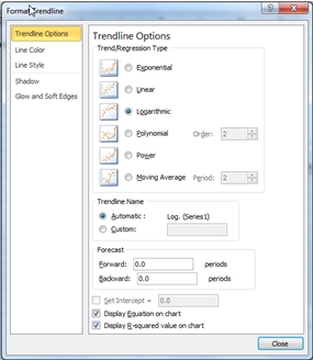
This produces the following chart.
This chart contains the plotted points of our x- and y-values, and has calculated a logarithmic trendline. The equation for that trendline is:
y = 20.050130*ln(x) + 8.010571
Which means that each y-value is calculated using this equation. For example, at x = 1.5
y = 20.050130*ln(1.5) + 8.010571
y = 16.1402
In XLeratorDB we have several functions that enable you to do precisely these types of calculations on the database. By using the SLOPE and INTERECPT function we can calculate the appropriate values for the logarithmic trendline
Let’s put our x- and y-values into a temporary table (just to keep things simple), and calculate the values.
SET NOCOUNT ON
SELECT *
INTO #xy
FROM (VALUES
(1,8.08526),
(2,21.94953),
(3,29.70361),
(4,35.92915),
(5,40.29423),
(6,44.01649)
) n(x,y)
SELECT ROUND(wct.INTERCEPT(y,LOG(x)), 6) as intercept
,ROUND(wct.SLOPE(y,LOG(x)), 6) as slope
FROM #xy
This produces the following result.
intercept slope
---------------------- ----------------------
8.010571 20.05013
These values equal the values produced by the EXCEL trendline.
We are now in a position to evaluate y at any value of x, using the coefficient and the exponent. Using the temporary table, we can simply evaluate y at x = 1.5.
SELECT ROUND(wct.SLOPE(y,LOG(x)), 6) * LOG(1.500000) + ROUND(wct.INTERCEPT(y,LOG(x)), 6) as y
FROM #xy
This produces the following result.
y
----------------------
16.1401991280327
This is exactly the result we would expect based on the logarithmic formula in the graph.
We can evaluate y at any x, with some very simple SQL. Let’s say we wanted to evaluate y at a number of points.
SELECT cast(xnew as float) as x
,ROUND(wct.SLOPE(y,LOG(x)), 6) * LOG(CAST(xnew as float)) + ROUND(wct.INTERCEPT(y,LOG(x)), 6) as y
FROM (VALUES
(0.5),(1),(1.5),(2),(2.5),(3),(3.5),(4),(4.5),(5),(5.5),(6),(6.5)
) m(xnew), #xy
GROUP BY xnew
This produces the following result.
x y
---------------------- ----------------------
0.5 -5.88712007936038
1 8.010571
1.5 16.1401991280327
2 21.9082620793604
2.5 26.382319291872
3 30.0378902073931
3.5 33.128631377518
4 35.8059531587208
4.5 38.1675183354259
5 40.2800103712323
5.5 42.1909918666324
6 43.9355812867535
6.5 45.5404479811599
As you can see, we are able to evaluate the function for values of x which are greater than the maximum value of x supplied as input to the function. In our #xy table, x is in the range [1, 6], yet we are able to return results for new x-values greater than 6. The same thing is true for values less than 1.
It is not possible to evaluate a logarithmic trendline where the x-values input to the calculation are less than or equal to zero, as the LOG function is undefined at those points. EXCEL will not allow you to generate a trendline for a range containing zero or negative x-values for this reason.
In this example, we will use the XLeratorDB number-generating function SERIESFLOAT to generate new x-values in the range [1, 6] in increments of .01. We will then take the results (which are not included here) and paste them into EXCEL and graph them. We can then compare the trendline values between EXCEL and SQL Server.
SELECT k.seriesvalue
,ROUND(wct.SLOPE(y,LOG(x)), 6) * LOG(k.seriesvalue) + ROUND(wct.INTERCEPT(y,LOG(x)), 6) as y
FROM (VALUES
(1,8.08526),
(2,21.94953),
(3,29.70361),
(4,35.92915),
(5,40.29423),
(6,44.01649)
) n(x,y)
CROSS APPLY wct.Seriesfloat(1,6.0,.01,NULL,NULL) k
GROUP BY k.SeriesValue
Here you can see a side-by-side comparison of the graphs.
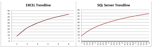
As you can see, the graphed results are identical.
In addition to the slope coefficient and the intercept, the EXCEL trendline function also gave us the option of displaying something called the R-squared value on the graph. We can calculate the R-squared value using the XLeratorDB RSQ function.
SELECT ROUND(wct.RSQ(y,LOG(x)), 6) as RSQ
FROM #xy
This produces the following result.
RSQ
----------------------
0.99984
This matches the EXCEL calculation. You can think of the R-squared value as a measure of how well the trendline fits through the existing y-values.
The real value in these functions, however, results in the fact that they are aggregate functions, so they can handle hundreds of thousands, even millions of rows of data in a single unit of work. Where this becomes handy is when these millions of rows are going to be grouped in some meaningful way. For example, if you wanted to analyze the price movements for every symbol traded on the NYSE over the preceding 14 trading days, you could do that using a logaritmic trendline and you can use the RSQ function to give you some measure of the variability of the result.
Here’s a very simple example. We will create a 3-column table holding the symbol, date, and closing price for the last 14 trading days. We will use the SLOPE and INTERCEPT functions to predict the price by creating a logarithmic trendline and we will also calculate the R-squared value. We will only use 5 different symbols for this example.
SET NOCOUNT ON
/*Create the table*/
CREATE TABLE #c(
sym char(3),
tdate datetime,
cprice float
)
/*Populate the table with data*/
INSERT INTO #c VALUES ('ABC','2011-04-01',6.64)
INSERT INTO #c VALUES ('DEF','2011-04-01',11.66)
INSERT INTO #c VALUES ('GHI','2011-04-01',10.66)
INSERT INTO #c VALUES ('JKL','2011-04-01',35.89)
INSERT INTO #c VALUES ('MNO','2011-04-01',113.79)
INSERT INTO #c VALUES ('ABC','2011-04-04',6.68)
INSERT INTO #c VALUES ('DEF','2011-04-04',11.77)
INSERT INTO #c VALUES ('GHI','2011-04-04',10.66)
INSERT INTO #c VALUES ('JKL','2011-04-04',35.89)
INSERT INTO #c VALUES ('MNO','2011-04-04',114.11)
INSERT INTO #c VALUES ('ABC','2011-04-05',6.74)
INSERT INTO #c VALUES ('DEF','2011-04-05',11.83)
INSERT INTO #c VALUES ('GHI','2011-04-05',10.74)
INSERT INTO #c VALUES ('JKL','2011-04-05',36.17)
INSERT INTO #c VALUES ('MNO','2011-04-05',115.08)
INSERT INTO #c VALUES ('ABC','2011-04-06',6.75)
INSERT INTO #c VALUES ('DEF','2011-04-06',11.9)
INSERT INTO #c VALUES ('GHI','2011-04-06',10.78)
INSERT INTO #c VALUES ('JKL','2011-04-06',36.39)
INSERT INTO #c VALUES ('MNO','2011-04-06',115.28)
INSERT INTO #c VALUES ('ABC','2011-04-07',6.78)
INSERT INTO #c VALUES ('DEF','2011-04-07',11.97)
INSERT INTO #c VALUES ('GHI','2011-04-07',10.87)
INSERT INTO #c VALUES ('JKL','2011-04-07',36.66)
INSERT INTO #c VALUES ('MNO','2011-04-07',116.29)
INSERT INTO #c VALUES ('ABC','2011-04-08',6.82)
INSERT INTO #c VALUES ('DEF','2011-04-08',12)
INSERT INTO #c VALUES ('GHI','2011-04-08',10.96)
INSERT INTO #c VALUES ('JKL','2011-04-08',36.89)
INSERT INTO #c VALUES ('MNO','2011-04-08',116.8)
INSERT INTO #c VALUES ('ABC','2011-04-11',6.88)
INSERT INTO #c VALUES ('DEF','2011-04-11',12.11)
INSERT INTO #c VALUES ('GHI','2011-04-11',10.99)
INSERT INTO #c VALUES ('JKL','2011-04-11',37.1)
INSERT INTO #c VALUES ('MNO','2011-04-11',117.53)
INSERT INTO #c VALUES ('ABC','2011-04-12',6.92)
INSERT INTO #c VALUES ('DEF','2011-04-12',12.21)
INSERT INTO #c VALUES ('GHI','2011-04-12',11.09)
INSERT INTO #c VALUES ('JKL','2011-04-12',37.31)
INSERT INTO #c VALUES ('MNO','2011-04-12',117.75)
INSERT INTO #c VALUES ('ABC','2011-04-13',6.98)
INSERT INTO #c VALUES ('DEF','2011-04-13',12.31)
INSERT INTO #c VALUES ('GHI','2011-04-13',11.19)
INSERT INTO #c VALUES ('JKL','2011-04-13',37.35)
INSERT INTO #c VALUES ('MNO','2011-04-13',118.33)
INSERT INTO #c VALUES ('ABC','2011-04-14',6.99)
INSERT INTO #c VALUES ('DEF','2011-04-14',12.32)
INSERT INTO #c VALUES ('GHI','2011-04-14',11.28)
INSERT INTO #c VALUES ('JKL','2011-04-14',37.61)
INSERT INTO #c VALUES ('MNO','2011-04-14',118.51)
INSERT INTO #c VALUES ('ABC','2011-04-15',7.04)
INSERT INTO #c VALUES ('DEF','2011-04-15',12.34)
INSERT INTO #c VALUES ('GHI','2011-04-15',11.33)
INSERT INTO #c VALUES ('JKL','2011-04-15',37.69)
INSERT INTO #c VALUES ('MNO','2011-04-15',118.94)
INSERT INTO #c VALUES ('ABC','2011-04-18',7.08)
INSERT INTO #c VALUES ('DEF','2011-04-18',12.43)
INSERT INTO #c VALUES ('GHI','2011-04-18',11.4)
INSERT INTO #c VALUES ('JKL','2011-04-18',38.04)
INSERT INTO #c VALUES ('MNO','2011-04-18',119.08)
INSERT INTO #c VALUES ('ABC','2011-04-19',7.14)
INSERT INTO #c VALUES ('DEF','2011-04-19',12.51)
INSERT INTO #c VALUES ('GHI','2011-04-19',11.4)
INSERT INTO #c VALUES ('JKL','2011-04-19',38.24)
INSERT INTO #c VALUES ('MNO','2011-04-19',120.23)
INSERT INTO #c VALUES ('ABC','2011-04-20',7.21)
INSERT INTO #c VALUES ('DEF','2011-04-20',12.53)
INSERT INTO #c VALUES ('GHI','2011-04-20',11.46)
INSERT INTO #c VALUES ('JKL','2011-04-20',38.52)
INSERT INTO #c VALUES ('MNO','2011-04-20',120.63)
/*Calculate the results*/
SELECT sym
,wct.SLOPE(y,LOG(x)) * LOG(CAST(15 as float)) + wct.INTERCEPT(y,LOG(x)) as [Predicted Value]
,ROUND(wct.RSQ(y,LOG(x)), 6) as [R-squared]
FROM (
SELECT sym
,ROW_NUMBER() OVER (PARTITION BY sym ORDER BY tdate) as x
,cprice as y
FROM #c
) n
GROUP by n.sym
/*Clean up*/
DROP TABLE #c
This produces the following result.
sym Predicted Value R-squared
---- ---------------------- ----------------------
ABC 7.0948356553739 0.850674
DEF 12.4529052726792 0.908654
GHI 11.3716815632026 0.858727
JKL 38.0609020871975 0.87536
MNO 119.742759218053 0.913539
You will notice that we used the ROW_NUMBER() function instead of passing dates to the aggregate functions. In general, because of the limits of floating point math, you will get the best results by reducing datetime values to values representing the elapsed time from some starting point (this also happens to be true with EXCEL trendline). In fact, in this example, we just used trading dates, so we were unconcerned about the weekends and we counted the number of days from a Friday to a Monday as 1 (and not 3).
Calculating logarithmic trendline values can be an important tool, either filling in the gaps between known x-values, or for predicting an outcome for some new x-value. And XLeratorDB makes it simple and efficient to do these calculations right on the database, where your data is.