Calculating Trendline Values in SQL Server Using XLeratorDB
Apr
26
Written by:
Charles Flock
4/26/2011 5:33 PM

In this posting we demonstrate how to replicate the EXCEL Polynomial Trendline in SQL Server.
Let’s start with the following data in EXCEL.
|
x
|
y
|
|
-2
|
-0.5
|
|
-1
|
0.8125
|
|
0
|
1
|
|
1
|
1.1875
|
|
2
|
2.5
|
|
3
|
6.0625
|
We then create a graph of the x- and y-values in EXCEL and add a trendline, using the Polynomial option, with an order of 3.
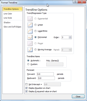
This produces the following chart.
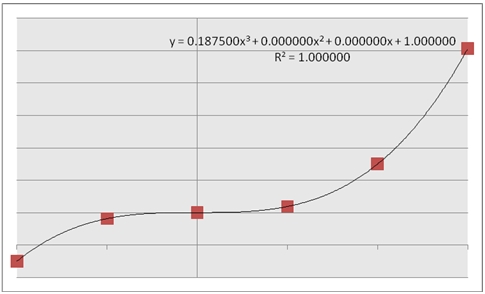
This chart contains the plotted points of our x- and y-values, and has calculated a trendline, which is a third-order polynomial which best fits the supplied values. The equation for that polynomial is:
0.1875x3 + 1
Which means that each y-value is calculated using this polynomial. For example, at x = 1.5
y = 0.1875(1.5)3 + 1
y = 1.6328125
In XLeratorDB we have added several functions that enable you to do precisely these types of calculations on the database. For example, the table-valued functions, POLYFIT and POLYFIT_q, will calculate the polynomial coefficients to a specified degree (degree being the equivalent of order in EXCEL), much like the equation displayed in the EXCEL graph.
Let’s put our x- and y-values into a temporary table (just to keep things simple), and calculate the coefficients.
SET NOCOUNT ON
SELECT *
into #xy
FROM (VALUES
(-2,-0.5),
(-1,0.8125),
(0,1),
(1,1.1875),
(2,2.5),
(3,6.0625)
)n(x,y)
SELECT coe_num,
ROUND(coe_val, 6) as coe_val
FROM wct.POLYFIT('#xy','x','y','',NULL,3)
This produces the following result.
coe_num coe_val
----------- ----------------------
4 1
3 0
2 0
1 0.1875
These values equal the values produced by the EXCEL trendline. The coefficients are numbered in the order in which they appear in the polynomial, starting from x3 and ending at x0. The polynomial would look like this:
y = 0.1875x3 + 0x2 + 0x1 + 1x0
This, of course, simplifies to
y = 0.1875x3 + 1
We are now in a position to evaluate y at any value of x, using a polynomial of degree 3. But, rather than using the output of the table-valued function, we can just use the aggregate function POLYVAL to simplify the whole process. Using the temporary table, we can simply evaluate y at x = 1.5.SELECT wct.POLYVAL(x,y,3,1.5) as y
FROM #xy
This produces the following result.
y
----------------------
1.6328125
This is exactly the result we would expect based on the polynomial.
We can evaluate y at any x, with some very simple SQL. Let’s say we wanted to evaluate y at a number of points.
SELECT xnew
,ROUND(wct.POLYVAL(x,y,3,xnew), 10) as Y
FROM (VALUES
(-2.5),(-2.25),(-2.0),(-1.75),(-1.50),(-1.25),(-1.0),(-0.75),
(-0.50),(-0.25),(0),(0.25),(0.5),(0.75),(1.0),(1.25),(1.50),(1.75)
,(2.0),(2.25),(2.50),(2.75),(3.0),(3.25),(3.5),(3.75),(4.0),(4.25)
) m(xnew), #xy
GROUP BY xnew
This produces the following result.
xnew Y
---------------------- ----------------------
-2.5 -1.9296875
-2.25 -1.1357421875
-2 -0.5
-1.75 -0.0048828125
-1.5 0.3671875
-1.25 0.6337890625
-1 0.8125
-0.75 0.9208984375
-0.5 0.9765625
-0.25 0.9970703125
0 1
0.25 1.0029296875
0.5 1.0234375
0.75 1.0791015625
1 1.1875
1.25 1.3662109375
1.5 1.6328125
1.75 2.0048828125
2 2.5
2.25 3.1357421875
2.5 3.9296875
2.75 4.8994140625
3 6.0625
3.25 7.4365234375
3.5 9.0390625
3.75 10.8876953125
4 13
4.25 15.3935546875
As you can see, we are able to evaluate the function for values of x which are greater than the maximum value of x supplied as input to the function. In our #xy table, x is in the range [-2, 3], yet the POLYVAL function is able to return results for new x-values greater than 3. The same thing is true for values less than -2.
In this example, we will use the XLeratorDB number-generating function SERIESFLOAT to generate new x values in the range [-2, 3] in increments of .01. We will then take the results (which are not included here) and paste them into EXCEL and graph them. We can then compare the trendline values between EXCEL and SQL Server.
SELECT k.SeriesValue as xnew
,ROUND(wct.POLYVAL(x,y,3,k.SeriesValue), 10) as y
FROM #xy, wct.SeriesFloat(-2,3,.01,NULL,NULL) k
GROUP BY k.SeriesValue
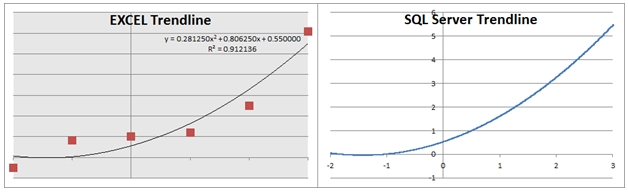
Here you can see a side-by-side comparison of the graphs.
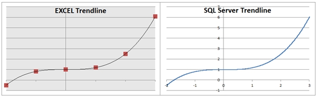
As you can see, the graphed results are identical.
In addition to the polynomial coefficients, the EXCEL trendline function also gave us the option of displaying something called the R-squared value on the graph. We can calculate the R-squared value using the XLeratorDB POLYRSQ function.SELECT ROUND(wct.POLYRSQ(x,y,3), 10) as [R-squared]
FROM #xy
This produces the following result.
R-squared
----------------------
1
You can think of the R-squared value as a measure of how well the polynomial fits through the existing y-values. The maximum value for R-squared is 1, so there is no point in calculating a polynomial with a degree higher than 3. In fact, if we set the degree to 5, we can see that we get exactly the same coefficients as when we set the degree to 3.
SELECT coe_num,
ROUND(coe_val, 6) as coe_val
FROM wct.POLYFIT('#xy','x','y','',NULL,5)
This produces the following result.
coe_num coe_val
----------- ----------------------
6 1
5 0
4 0
3 0.1875
2 0
1 0
This produces the following polynomial.
y = 0x5 + 0x4 + 0.1875x3 + 0x2 + 0x1 + 1x0
y = 0.1875x3 + 1x0
This is exactly the same polynomial as we had when we set the degree to 3.
Let’s see what happens when we use a second degree polynomial.
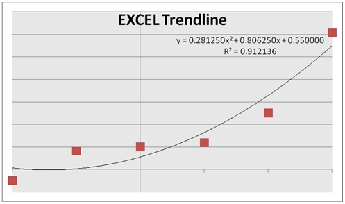
We can immediately observe that the trendline no longer goes through the y-values on the graph. We can also see that the R-squared value is less than 1 (0.912136). Let’s see what the R-squared value is in SQL Server.
SELECT ROUND(wct.POLYRSQ(x,y,2), 6) as [R-squared]
FROM #xy
This produces the following result.
R-squared
----------------------
0.912136
The SQL Server result matches the EXCEL result.
Let’s calculate the coefficients.
SELECT coe_num,
ROUND(coe_val, 6) as coe_val
FROM wct.POLYFIT('#xy','x','y','',NULL,2)
This produces the following result.
coe_num coe_val
----------- ----------------------
3 0.55
2 0.80625
1 0.28125
Once again, the SQL Server results match the EXCEL results.
Here, we again produce all the y values for x in the range [-2, 3] in increments of .01, graph the results in EXCEL and compare them to the trendline.
SELECT k.SeriesValue as xnew
,ROUND(wct.POLYVAL(x,y,2,k.SeriesValue), 10) as y
FROM #xy, wct.SeriesFloat(-2,3,.01,NULL,NULL) k
GROUP BY k.SeriesValue
This is a comparison of the 2 graphs.
We can see that the trendlines are the same.
If we set the degrees to 1, we will be creating the polynomial coefficients for the following equation:
y = mx + b
This is immediately recognizable as the formula for a line. Let’s see what EXCEL produces.
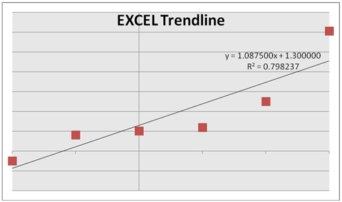
We can also see that as the number of degrees decreases, the R-squared value decreases. Let’s see what the polynomial coefficients are in SQL Server.
SELECT coe_num,
ROUND(coe_val, 6) as coe_val
FROM wct.POLYFIT('#xy','x','y','',NULL,1)
This produces the following result.
coe_num coe_val
----------- ----------------------
2 1.3
1 1.0875
These results agree with EXCEL. It is also interesting to note, that for a first-degree polynomial, the coefficients represent the slope and y-intercept of the least squares fitted line, which can be calculated directly using the XLeratorDB SLOPE and INTERCEPT functions.
SELECT wct.SLOPE(y,x) as [1]
,wct.INTERCEPT(y,x) as [2]
FROM #xy
This produces the following result.
1 2
---------------------- ----------------------
1.0875 1.3
As in the previous examples, we can use the POLYVAL function to evaluate y for any value of x. This will produce the same result as using the FORECAST function, which is computationally more efficient.SELECT wct.POLYVAL(x,y,1,1.5) as POLYVAL
,wct.FORECAST(1.5,y,x) as FORECAST
FROM #xy
This produces the following result.
POLYVAL FORECAST
---------------------- ----------------------
2.93125 2.93125
The real value in the POLYVAL function, however, results in the fact that it is an aggregate function, so it can handle hundreds of thousands, even millions of rows of data in a single unit of work. Where this becomes handy is when these millions of rows are going to be grouped in some meaningful way. For example, if you wanted to analyze the price movements for every symbol traded on the NYSE over the preceding 14 trading days, you could do that using POLYVAL and you can use the POLYRSQ function to give you some measure of the variability of the result.
Here’s a very simple example. We will create a 3-column table holding the symbol, date, and closing price for the last 14 trading days. We will use the POLYVAL function to predict the price by creating a 4th degree polynomial and we will also calculate the R-squared value. We will only use 5 different symbols for this example.
SET NOCOUNT ON
/*Create the table*/
CREATE TABLE #c(
sym char(3),
tdate datetime,
cprice float
)
/*Populate the table with data*/
INSERT INTO #c VALUES ('ABC','2011-04-01',6.64)
INSERT INTO #c VALUES ('DEF','2011-04-01',11.66)
INSERT INTO #c VALUES ('GHI','2011-04-01',10.66)
INSERT INTO #c VALUES ('JKL','2011-04-01',35.89)
INSERT INTO #c VALUES ('MNO','2011-04-01',113.79)
INSERT INTO #c VALUES ('ABC','2011-04-04',6.68)
INSERT INTO #c VALUES ('DEF','2011-04-04',11.77)
INSERT INTO #c VALUES ('GHI','2011-04-04',10.66)
INSERT INTO #c VALUES ('JKL','2011-04-04',35.89)
INSERT INTO #c VALUES ('MNO','2011-04-04',114.11)
INSERT INTO #c VALUES ('ABC','2011-04-05',6.74)
INSERT INTO #c VALUES ('DEF','2011-04-05',11.83)
INSERT INTO #c VALUES ('GHI','2011-04-05',10.74)
INSERT INTO #c VALUES ('JKL','2011-04-05',36.17)
INSERT INTO #c VALUES ('MNO','2011-04-05',115.08)
INSERT INTO #c VALUES ('ABC','2011-04-06',6.75)
INSERT INTO #c VALUES ('DEF','2011-04-06',11.9)
INSERT INTO #c VALUES ('GHI','2011-04-06',10.78)
INSERT INTO #c VALUES ('JKL','2011-04-06',36.39)
INSERT INTO #c VALUES ('MNO','2011-04-06',115.28)
INSERT INTO #c VALUES ('ABC','2011-04-07',6.78)
INSERT INTO #c VALUES ('DEF','2011-04-07',11.97)
INSERT INTO #c VALUES ('GHI','2011-04-07',10.87)
INSERT INTO #c VALUES ('JKL','2011-04-07',36.66)
INSERT INTO #c VALUES ('MNO','2011-04-07',116.29)
INSERT INTO #c VALUES ('ABC','2011-04-08',6.82)
INSERT INTO #c VALUES ('DEF','2011-04-08',12)
INSERT INTO #c VALUES ('GHI','2011-04-08',10.96)
INSERT INTO #c VALUES ('JKL','2011-04-08',36.89)
INSERT INTO #c VALUES ('MNO','2011-04-08',116.8)
INSERT INTO #c VALUES ('ABC','2011-04-11',6.88)
INSERT INTO #c VALUES ('DEF','2011-04-11',12.11)
INSERT INTO #c VALUES ('GHI','2011-04-11',10.99)
INSERT INTO #c VALUES ('JKL','2011-04-11',37.1)
INSERT INTO #c VALUES ('MNO','2011-04-11',117.53)
INSERT INTO #c VALUES ('ABC','2011-04-12',6.92)
INSERT INTO #c VALUES ('DEF','2011-04-12',12.21)
INSERT INTO #c VALUES ('GHI','2011-04-12',11.09)
INSERT INTO #c VALUES ('JKL','2011-04-12',37.31)
INSERT INTO #c VALUES ('MNO','2011-04-12',117.75)
INSERT INTO #c VALUES ('ABC','2011-04-13',6.98)
INSERT INTO #c VALUES ('DEF','2011-04-13',12.31)
INSERT INTO #c VALUES ('GHI','2011-04-13',11.19)
INSERT INTO #c VALUES ('JKL','2011-04-13',37.35)
INSERT INTO #c VALUES ('MNO','2011-04-13',118.33)
INSERT INTO #c VALUES ('ABC','2011-04-14',6.99)
INSERT INTO #c VALUES ('DEF','2011-04-14',12.32)
INSERT INTO #c VALUES ('GHI','2011-04-14',11.28)
INSERT INTO #c VALUES ('JKL','2011-04-14',37.61)
INSERT INTO #c VALUES ('MNO','2011-04-14',118.51)
INSERT INTO #c VALUES ('ABC','2011-04-15',7.04)
INSERT INTO #c VALUES ('DEF','2011-04-15',12.34)
INSERT INTO #c VALUES ('GHI','2011-04-15',11.33)
INSERT INTO #c VALUES ('JKL','2011-04-15',37.69)
INSERT INTO #c VALUES ('MNO','2011-04-15',118.94)
INSERT INTO #c VALUES ('ABC','2011-04-18',7.08)
INSERT INTO #c VALUES ('DEF','2011-04-18',12.43)
INSERT INTO #c VALUES ('GHI','2011-04-18',11.4)
INSERT INTO #c VALUES ('JKL','2011-04-18',38.04)
INSERT INTO #c VALUES ('MNO','2011-04-18',119.08)
INSERT INTO #c VALUES ('ABC','2011-04-19',7.14)
INSERT INTO #c VALUES ('DEF','2011-04-19',12.51)
INSERT INTO #c VALUES ('GHI','2011-04-19',11.4)
INSERT INTO #c VALUES ('JKL','2011-04-19',38.24)
INSERT INTO #c VALUES ('MNO','2011-04-19',120.23)
INSERT INTO #c VALUES ('ABC','2011-04-20',7.21)
INSERT INTO #c VALUES ('DEF','2011-04-20',12.53)
INSERT INTO #c VALUES ('GHI','2011-04-20',11.46)
INSERT INTO #c VALUES ('JKL','2011-04-20',38.52)
INSERT INTO #c VALUES ('MNO','2011-04-20',120.63)
/*Calculate the results*/
SELECT sym
,ROUND(wct.POLYVAL(x,y,4,14), 2) as POLYVAL
,ROUND(wct.POLYRSQ(x,y,4), 6) as POLYRSQ
FROM (
SELECT sym
,ROW_NUMBER() OVER (PARTITION BY sym ORDER BY tdate) - 1 as x
,cprice as y
FROM #c
) n
GROUP by n.sym
/*Clean up*/
DROP TABLE #c
This produces the following result.
sym POLYVAL POLYRSQ
---- ---------------------- ----------------------
ABC 7.28 0.995338
DEF 12.57 0.991893
GHI 11.45 0.996454
JKL 39.05 0.996317
MNO 121.99 0.994015
You will notice that we used the ROW_NUMBER() function instead of passing dates to the POLYVAL function. In general, because of the limits of floating point math, you will get the best results by reducing datetime values to values representing the elapsed time from some starting point (this also happens to be true with EXCEL trendline). In fact, in this example, we just used trading dates, so we were unconcerned about the weekends and we counted the number of days from a Friday to a Monday as 1 (and not 3).
Calculating trendline values can be an important tool, either filling in the gaps between known x-values, or for predicting an outcome for some new x-value. And XLeratorDB makes it simple and efficient to do these calculations right on the database, where your data is.