Time Value of Money Problems in EXCEL
Nov
18
Written by:
Charles Flock
11/18/2010 6:09 PM

How a simple table-valued function led to a deep dive into the time value of money functions in EXCEL where we discover that the EXCEL IPMT and PPMT functions are broken for payments made at the beginning of the period—even in EXCEL 2010.
In the recently released XLeratorDB/finance release 1.06, we added a new table-valued function, PMTSCHED, which automatically creates an amortization schedule when supplied with the principal amount, the residual value, the number of payments, and the payment amount for a loan or a lease. The idea behind the function is that this information is normally what’s most readily available for a loan and that the loan rate could be easily calculated. Here’s a very simple example: you have a $3,000 loan with 15 monthly payments of $215.
SELECT *
FROM wct.PMTSCHED(
3000 --Loan amount
,215 --payment amount
,15 --number of periods
,0 --Future value
,0 --payment type
)
This produces the following result.
num_pmt amt_prin_init amt_int_pay amt_prin_pay amt_prin_end
----------- ---------------------- ---------------------- ---------------------- ----------------------
1 3000 27.5380518582788 187.461948141721 2812.53805185828
2 2812.53805185828 25.8172729165199 189.18272708348 2623.3553247748
3 2623.3553247748 24.0806983329421 190.919301667058 2432.43602310774
4 2432.43602310774 22.3281831223758 192.671816877624 2239.76420623012
5 2239.76420623012 20.5595809602273 194.440419039773 2045.32378719034
6 2045.32378719034 18.7747441787178 196.225255821282 1849.09853136906
7 1849.09853136906 16.9735237545829 198.026476245417 1651.07205512364
8 1651.07205512364 15.1557692966344 199.844230703366 1451.22782442028
9 1451.22782442028 13.3213290331696 201.67867096683 1249.54915345345
10 1249.54915345345 11.4700497993217 203.529950200678 1046.01920325277
11 1046.01920325277 9.60177702429792 205.398222975702 840.620980277068
12 840.620980277068 7.71635471841364 207.283645281586 633.337334995482
13 633.337334995482 5.81362546010496 209.186374539895 424.150960455587
14 424.150960455587 3.89343038279912 211.106569617201 213.044390838386
15 213.044390838386 1.95560916161412 213.044390838386 0
(15 row(s) affected)
This returns a table showing the payment number, the principal amount at the beginning of the period, the interest paid during the period, the principal paid during the period, and the ending principal amount. The function automatically figures out the rate.
There are couple of axioms that reveal themselves in this presentation. The first is that the total interest on the loan is equal to the payment amount multiplied by the number of payments less the difference between the loan amount and the future value.
Total Interest = pmt * numpmts – (PV-FV)
The second axiom is that for any row in the in amortization table, the beginning principal balance is equal to the present value of the future cash flows
Amt_prin_init = PV(r, numpmts-num_pmt+1,-pmt, fv, pay_type)
As you can see, I have introduced a new variable, r, which represents the rate of interest for the loan. The rate of interest is calculated by the RATE function as:
R = RATE(numpmts,-pmt,pv,fv,pay_type)
These axioms are logical extensions of this relationship, which turns up repeatedly (e.g. PV, PMT, FV) in the EXCEL documentation:
“Microsoft EXCEL solves for one financial argument in terms of the other. If the rate is not 0, then”

I will spend the rest of this article demonstrating that EXCEL does not, in fact, adhere to this rule, and that the IPMT and PPMT functions, when the pay_type is equal to 1, return incorrect results. And, I will use EXCEL itself, to prove this.
To make the demonstration clearer, we will use an extreme example. We have a 100,000 loan, with a rate of 30%, that has 3 payments, and we will start off with a pay_type of 0 (meaning that it pays at the end). I am going to enter the loan parameters into a spread sheet and then create a loan amortization table. Here are the formulae:
And here are the results
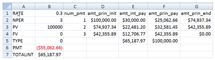
Notice that the spreadsheet calculates the interest and principal payment amounts without using the IPMT or the PPMT functions. The only functions that are used are PMT, PV, and SUM. The rate value (found in B1) is only used in the calculation of the PV amounts and is not used for the calculation of the interest column (E) at all. Let’s call this method, the PV method.
Notice that our axioms are satisfied. The sum of the interest amounts (E5) is equal to the total interest as calculated in B7. And that we have calculated both the beginning and the ending principal balances using the PV function. Thus, there was no need to invoke the IPMT and PPMT function in creating the amortization schedule.
What about a loan which includes a future value? Since we are using an extreme example, let’s set the FV equal to -90000 and set the PV = 0. We should not have to change any of our formulae (otherwise they would not be axiomatic). Here’s what the results look like:
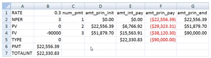
Again, our axioms are satisfied.
Let’s combine the two examples, and see what we get.
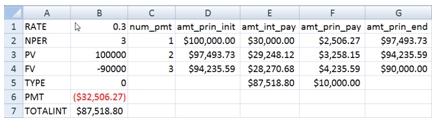
Axioms satisfied again. It’s also interesting to note the values in columns E and F are the sum of the first two examples.
To this point, we haven’t really talked about IPMT and PPMT. This is because, when the pay_type is 0 (pay at the end), these functions produce correct results. So, we can just add 2 more columns to our spreadsheet with the IPMT and PPMT results (for consistency sake, I am using IPMT*-1 and PPMT*-1).
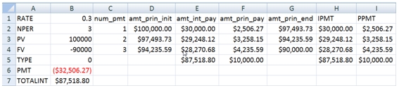
Thus, we can see that the IPMT and PPMT agree with the PV method, which is what we should expect.
The pay_type identifies whether the payment is made at the beginning of the period or at the end of the period. To calculate the payment amount for a loan that pays at the beginning, you simple take the PMT calculation for pay-at-the-end and divide by 1 plus the rate. Symbolically:
PMT(rate,nper,pv,fv,1) = PMT(rate,nper,pv,fv,0)/(1+rate)
So, let’s look at our example and see what happens when we change the pay_type to 1.
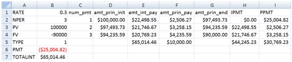
As you can see, under the PV method, our axioms still hold true. The total interest is still correct and the principal balance is still the present value of the future cash flows.
But look at the IPMT and the PPMT calculations. The sum of IPMT (H5) is $44,245.23 vs. the $65,014.46 that is calculated in B7. The sum of PPMT (I5) is $30,769.23, which doesn’t really seem to be related to anything having to do with the loan transaction, though it does equal the sum of the payments less the sum of IPMT values.
For the pay-at-the-end example we saw that the third example was the sum of the first two examples, so it should be possible to decompose this transaction into two streams of payments associated with the PV and the FV of the transaction.
Let’s look at the PV first.
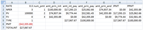
The total in column E and the total in column H are the same and agree with the total interest calculation; and the total in column F and the total in column I are the same and are equal to the PV amount. But the rows do not agree.
The IPMT function calculates a zero amount for the first period and applies the entire payment amount to PPMT. Our calculation shows $17,293.23 in interest for the first period and a $25,062.66 principal payment.
The payment amount for the pay-at-the-end example is $55,062.66. Dividing that amount by 1 + rate (1.3) gives us $42.335.89. And remember that the first payment consisted of $30,000 in interest and $25,062.66 in principal. And, since the formulae are all related, it’s quite easy to see that $30,000 in interest is equal to the rate multiplied by the PV ($100,000 * .3), though we didn’t calculate it that way.
The $17,293.23 can be calculated in almost exactly the same way. Since the loan is pay-at-the-beginning, the first period interest is calculated as (PV – amt_prin_pay) * rate. This amount is then divided by 1.3.
$17,293.23 = ((100,000 – 25,062.66) * .3)/1.3
Let’s just review that calculation again. We calculated the interest amount for the first period as $22,481.20 and then discounted it to the beginning of the period using our rate of 30%.
Of course, that’s not the calculation that’s in our worksheet; it’s just using the present value calculations, since all the calculations should be related. You can also see that, over time, the interest payment amounts decline and the principal payment amounts increase, which is exactly what you would expect for an amortizing loan.
What about the EXCEL calculation? It looks like it’s implemented with a rule along the line that if period number is equal to 1, then set the IPMT amount to zero. And, since the IPMT is zero, then the entire payment is applied to principal. So what’s the problem with that rule?
First, look at the payments. The interest payments increase and then decrease, rather than decreasing smoothly. The principal payment decreases and then increases rather than increasing smoothly. Second, the principal balance at any point in time is no longer equal to the present value of the future cash flows. Third, when we add FV to the mix, the total interest and principal amounts are wrong.
Now, let’s look at the FV calculation.
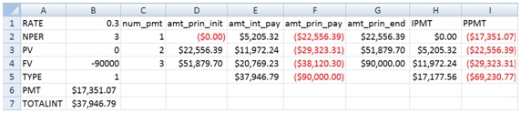
The PV method once again calculates interest payments so that their sum (E5) equals the total interest calculated in B7. The sum of the EXCEL calculations (H5) is off by $20,769.23, which is the interest for the last period as shown in E7.
Once again, this difference seems to be entirely due to the inferred rule that if it’s the first period, then the interest payment must be zero. However, we can actually use another EXCEL function, FV, to demonstrate that that EXCEL calculation is wrong. Go to cell J2 and enter the following formula.
=-FV($B$1,C2,$B$6,0,$B$5)
Copy the formula to J3:J4. This is what the results should look like:
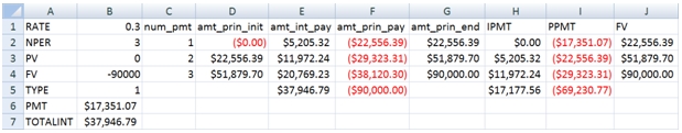
As you can see, the FV calculation (column J) agrees with the PV method (column G), which is exactly what we would expect since the formulae are related. Clearly, by forcing the interest amount in the first period to be zero, all subsequent IPMT and PPMT calculations are incorrect.
One of the consequences of this, of course, is that the CUMPRINC and the CUMIPMT functions are incorrect as well. Of course, since these functions do not actually accept FV as input, you would need to use something like the PV method as a work-around anyway. Clearly, you can use the formulae in this article to work around this limitation in EXCEL, and it’s really not too burdensome.
I also performed the same analysis in OpenOffice and got exactly the same results. I wonder what that says about the benefits of open source development.
I have laid out my case. I think that the math is compelling and I believe that the math is consistent with Microsoft’s own documentation. So, why can’t I find any other article about this anywhere on the web? I guess that leaves open the possibility that I am wrong and that all the developers at Microsoft and OpenOffice have it right; making my entire analysis specious. Here is the excel spreadsheet for download. Take a look for yourself and tell me what you think.